Simple Harmonic Oscillations
We’ve all seen simple harmonic motion, it is the motion you observe when you watch a grandfather clock tick back and forth, or when a spring oscillates by contracting and extending. It is something that is periodic in motion and moves at a frequency determined either by the system or a driving force. In this post we will discuss how we can solve the equations of motion for oscillators.
Linear differential equations show up in many different places throughout physics. The term linear just tells us that the highest degree polynomial in our equation is 0 or 1. Some of the interesting places this type of equation pops up is in pendulums, springs, circuits, and pretty much anything that has to do with simple harmonic motion.
The way to arrive at the differential equation differs from system to system, it can range from using restoring forces and torques to Kirchhoff’s current law. However different these systems may seem they are based on the same underlying mathematical concept.
The Simplest Case
Let’s take for example an idealized pendulum system without a damping or driving force in a conservative gravitational field.
An important relationship to note is $T = \frac{2\pi}{\omega}$. $T$ is the period, the time it takes to complete one full oscillation. Frequency $f = \frac{1}{T}$ tells us how many times it oscillates per second. Another relation can be seen that $\omega = 2\pi f$. In this context $\omega$ is the variable we use to denote angular frequency; however, it is also sometimes used to denote angular velocity. These two are not to be confused as angular velocity is a vector quantity with which the pendulum rotates with, and angular frequency is a scalar quantity telling us the number of radians per second of the oscillation. Because of this we will use another variable to denote angular velocity.
Here are the variables:
- $E$: total mechanical energy
- $T$: kinetic energy
- $V$: potential energy
- $m$: mass
- $l$: distance from the axis of rotation to center of mass
- $J = ml^2$: moment of inertia
- $\vartheta$: angle of displacement from equilibrium
- $\dot{\vartheta}$: angular velocity
- $\ddot{\vartheta}$: angular acceleration
A dot above a variable denotes it is the first time derivative of the variable, and two dots the second time derivative.
Since we know energy is conserved (constant) in this system it implies
\[\frac{d}{dt}E = 0 \implies \frac{d}{dt}[T + V] = 0\]Where:
\[T = \frac{1}{2}J\dot{\vartheta}^2 = \frac{1}{2}ml^2\dot{\vartheta^2}\] \[V = mgl(1-\cos\vartheta)\]Taking the time derivative of $T$ and $V$ we get this homogeneous linear differential equation:
\[ml^2\ddot{\vartheta}\dot{\vartheta} + mgl\sin\vartheta\dot{\vartheta} = 0\]Which can be simplified to:
\[\ddot{\vartheta} + \frac{g}{l}\vartheta = 0\]First order Taylor expansion gives us:
\[\sin\vartheta \approx \vartheta\]Using the auxiliary equation (will discuss below) and a little bit of algebra we arrive at:
\[\vartheta = A\cos(\omega_0t + \varphi_0)\]Where:
\[\omega_0^2 = \frac{g}{l}\]The amplitude $A$ and phase shift $\varphi_0$ are constants determined by the initial conditions. $\omega_0$ corresponds to the natural frequency of the oscillator.
That was the simplest example of how the linear differential equation shows up in simple harmonic oscillations, now we will dive deeper into what happens if we have damping and also if we have a driving force.
Damped Oscillations
First let’s start with that of a damped system - a system which has a force acting against the motion. Whatever the system may be, eventually one arrives at a homogeneous linear differential equation of the form:
\[m\ddot{x} + b\dot{x} + kx = 0\]Where $b$ is the damping constant and $k$ the restoring force constant.
It is always good to move variables around to get an isolated $\ddot{x}$, leading us to:
\[\ddot{x} + \gamma\dot{x} + \omega_0^2x = 0\]Where:
\[\gamma = \frac{b}{m}\] \[\omega_0^2 = \frac{k}{m}\]There are multiple ways to solve linear differential equations, but for this we will use the auxiliary equation. The auxiliary equation is an ‘ansatz’ (German word for approach) or educated guess based off what we know about the equation. Since it’s linear the auxiliary equation leverages the power of Euler’s constant and its ease of differentiation. We know that $\frac{d}{dt}e^{\lambda t} = \lambda e^{\lambda t}$. Using it as the approach to our equation we get:
\[\lambda^2 e^{\lambda t} + \gamma\lambda e^{\lambda t} + \omega_0^2 e^{\lambda t} = 0\]Removing the $e^{\lambda t}$ we get:
\[\lambda^2 + \gamma\lambda + \omega_0^2 = 0\]Which can be easily solved using the quadratic equation:
\[\lambda = - \frac{\gamma}{2} \pm \sqrt{(\frac{\gamma}{2})^2 - \omega_0^2}\]There are three scenarios:
- Under-damped when $\frac{\gamma}{2} < \omega_0$
- Critically-damped when $\frac{\gamma}{2} = \omega_0$
- Over-damped when $\frac{\gamma}{2} > \omega_0$
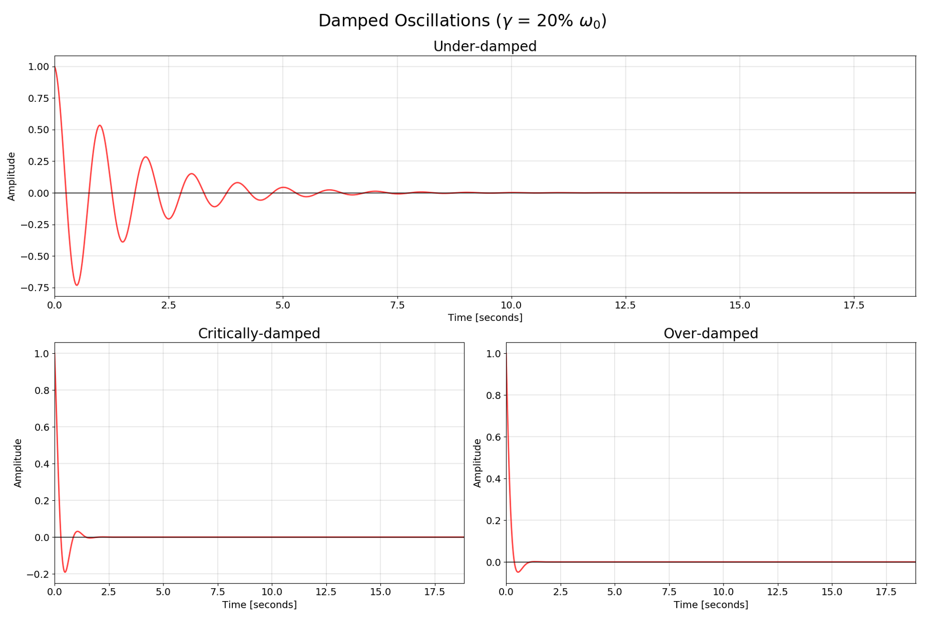
I will focus on the under-damped case which still oscillates, but with decreasing amplitude, and eventually stops as $t \implies \infty$.
\[\frac{\gamma}{2} < \omega_0 \implies \lambda = - \frac{\gamma}{2} \pm i\sqrt{\omega_0^2 - (\frac{\gamma}{2})^2}\] \[\omega' = \sqrt{\omega_0^2 - (\frac{\gamma}{2})^2}\]Substituting $\lambda$ in and manipulating the equation a bit we get the complimentary (homogeneous) solution:
\[x_c = c e^{-\frac{\gamma}{2} t}\cos(\omega't + \varphi_0)\]Where $c$ and $\varphi_0$ are constants set by the initial conditions.
Here’s some plots illustrating the three different scenarios:
Driven Oscillations With Damping
Now let’s work on the non-homogeneous equation with a driving force. Let’s assume the equation is the same as in the previous where we solved with damping, but it has an extra term from the driving force in the equation (which is why it’s called non-homogeneous).
\[\ddot{x} + \gamma\dot{x} + \omega_0^2x = \frac{F}{m}\cos\omega t\]Where $F =$ driving force and $\omega =$ the angular frequency of the driving force.
To solve this equation we will leverage Euler’s identity:
\[e^{i\varphi} = \cos\varphi + i\sin\varphi\]We can create a new equation where our equation is the real part of the new equation and our solution is the real part of the new solution.
New equation:
\[\ddot{z} + \gamma\dot{z} + \omega_0^2z = \frac{F}{m}e^{i\omega t}\]Using an ansatz of $Ae^{i\omega t}$ yields:
\[-\omega^2 Ae^{i\omega t} + i\omega\gamma Ae^{i\omega t} + \omega_0^2Ae^{i\omega t} = \frac{F}{m}e^{i\omega t}\]With some rearranging we get:
\[(\omega_0^2 - \omega^2 + i\omega\gamma)A = \frac{F}{m}\]For simplification let $I = (\omega_0^2 - \omega^2) + i\omega\gamma$
The angle of $I$ in the complex plane $\varphi = \arctan\frac{\omega\gamma}{\omega_0^2 - \omega^2}$
The distance to $I$ in the complex plane $|I| = \sqrt{(\omega_0^2 - \omega^2)^2 + (\omega\gamma)^2}$
Leads us to:
\[A = \frac{F}{mI}\]The beauty of complex numbers lets us represent $I$ in exponential form using the angle and distance in the complex plane calculated above. Therefore:
\[I = |I|e^{i\varphi} \implies A = \frac{F}{m|I|}e^{-i\varphi}\]Thus we obtain our particular solution to our new equation:
\[z_p = e^{i(\omega t - \varphi)}\]Since we already know the solution to our original equation is the real part of$z_p$, we can extract it from Euler’s identity and finish up the complete solution to our damped and driven oscillator:
\[x_p = \cos(\omega t - \varphi)\]The complete solution is the the sum of the complimentary and particular solutions, thus we now have:
\[x =c e^{-\frac{\gamma}{2} t}\cos(\omega't + \varphi_0) +\frac{F}{m|I|}\cos(\omega t - \varphi)\]$x_c$ is called the transient solution which is determined by the system’s initial conditions and $x_p$ is called the steady-state solution, because as $t \implies \infty$ $x_c$ will tend to zero and $x_p$ will remain.
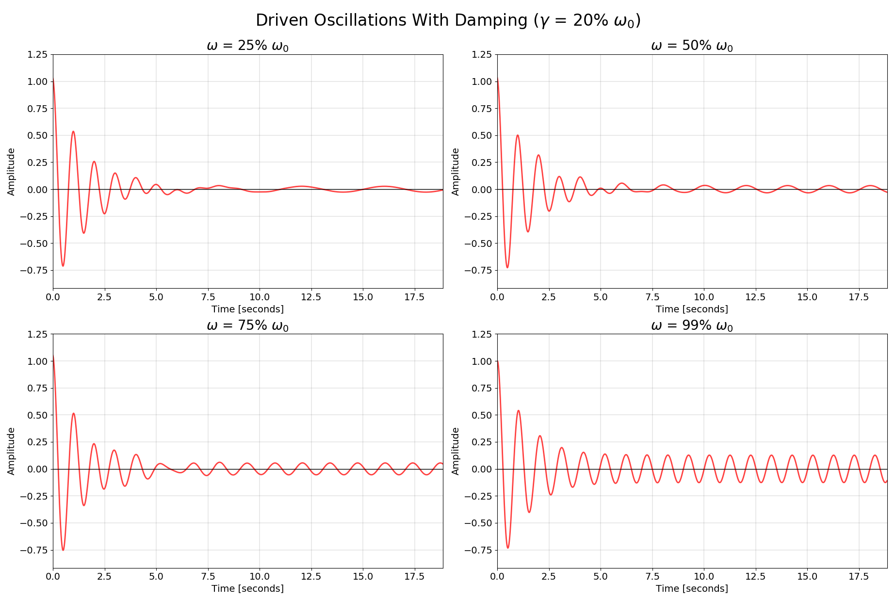
The most interesting behavior occurs when $\omega = \omega_0$. This is called the resonance. Because $|I|$ is downstairs, when $\omega = \omega_0$ it decreases the size of the denominator, increasing the overall amplitude of oscillations. A good way to describe it is that the resonance frequency is the frequency at which the transfer of energy is particularly efficient.
These charts clearly show when the steady state part of the solution takes over as well as the increase in amplitude near resonance frequency (bottom right):
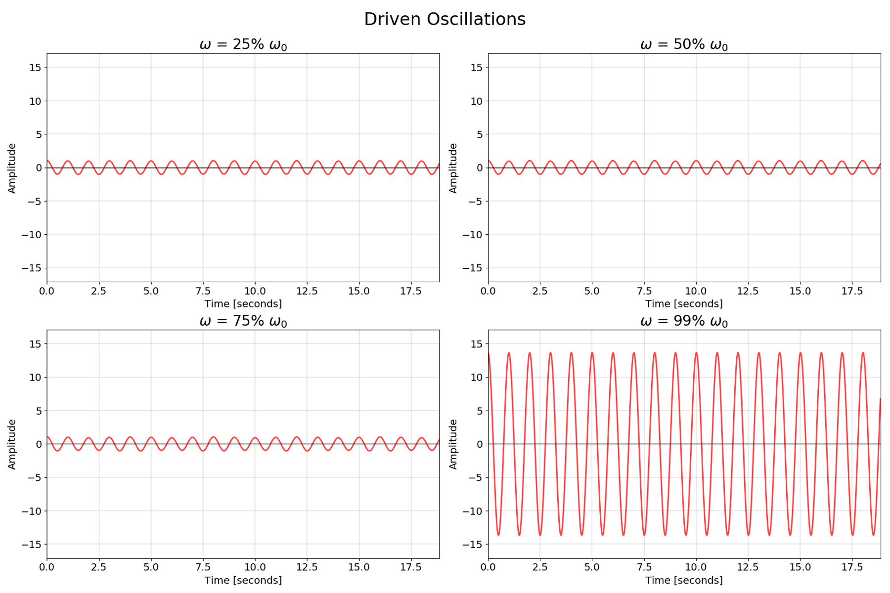
Bonus chart showing resonance in a driven system without damping:
Oscillations are one of my favorite topics in physics, and this post is just the tip of the iceberg. If you have any questions or comments feel free to contact me and I’ll be happy to discuss this with you!