Simulating Magnetism Part 1: Statistical Physics and the Ising Model
In physics we are often interested in modeling systems that are too complex to be modeled exactly so we have to turn to statistical modeling to to get an understanding of some of the macroscopic properties of the system without having to worry too much about the exact microscopic composition. Naturally computational physics has helped us understand a lot about statistical physics because of our ability to simulate and analyze systems with today’s ever increasing computational power. In this post we’ll cover some of the necessary concepts of statistical physics to use as a foundation for our journey through simulating magnetism.
The Ising Model
One model we have learned a lot from is the Ising model of ferromagnetism. To get an idea of how it works let us consider a lattice where at each site $i$ of the lattice we have a spin $\sigma_i$ that can take on a value of $\pm 1$ corresponding to the spin pointing up or down. The Hamiltonian (energy) of the system in configuration ${\sigma}$ using the mean field approximation (i.e. we assume each spin is subject to an effective magnetic field $h$) and assuming a homogeneous coupling constant ($J_{ij} = J$) is then given by:
\[H(\{\sigma\}) = -J \sum_{\langle i j \rangle} \sigma_i \sigma_j - h \sum_i \sigma_i\]Where the sum over $\langle i j \rangle$ is summing over every neighboring spin pair.
However, we will be examining the case where there is no external magnetic field, thus our Hamiltonian reduces to:
\[H(\{\sigma\}) = -J \sum_{\langle i j \rangle} \sigma_i \sigma_j\]If $J > 0$ the energy is lowest when all spin pairs are aligned and highest when anti-aligned.
The magnetization of the system is given by:
\[M = \sum_i \sigma_i\]The Canonical Ensemble
With the energy and magnetization we can now use statistical methods to obtain information about their probability distributions. To continue we must first understand the concept of a statistical ensemble. We can think of it as a virtual collection of all of the possible configurations of the system. Some of the configurations might have the same macroscopic properties but have different microscopic configurations. To get an idea of this we can think of a simple two-spin system where the energy is the same if both spins are up or down, thus two different configurations have the same energy.
In statistical physics we have three main equilibrium ensembles we use to model systems where the probability distribution is not explicitly dependent on time:
- Microcanonical - used for an isolated system whose energy and number of particles remain constant
- Canonical - used for a system in thermal equilibrium with a reservoir at a fixed temperature with which it is allowed to exchange energy, but the number of particles remains constant
- Grand Canonical - used for a system in thermal equilibrium with a reservoir where both energy and particles can be exchanged with the reservoir
Here we will be using the canonical ensemble so let’s clarify exactly what that is. The canonical ensemble is a way of representing a system at a constant temperature $T$ with a fixed number of particles $N$, but we allow the energy to fluctuate. This ensemble is characterized by it’s partition function $Z$, which contains a lot of information about the system. For a discrete system like the Ising model we have:
\[Z = \sum_{\{\sigma\}} e^{-\beta H(\{\sigma\})}\]Where $\beta = \frac{1}{k_B T}$ and $k_B$ is Boltzmann’s constant.
From this we can obtain some interesting quantities such as the free energy $F$ which is a measure of the amount of useful work one could extract from the system, or the average energy $E$.
\[\begin{align*} \begin{split} F &= -\frac{\log Z}{\beta} \\ E &= -\frac{\partial \log Z}{\partial \beta} \end{split} \end{align*}\]When the system is in thermal equilibrium the probability of the system to be in configuration ${\sigma}$ is given by:
\[P_{eq}(\{\sigma\}) = \frac{e^{-\beta H(\{\sigma\})}}{Z}\]Therefore, we see that the probability is dependent on both the internal energy of the system as well as the temperature.
1D Ising Model Solution
Let us think of a 1D Ising model, i.e. $N$ spins lined up with interactions between nearest-neighbors (i.e. only spins directly next to each other interact) and free boundary conditions (i.e. the first spin only interacts with the second and the last spin only interacts with the second to last, in contrast with periodic boundary conditions where the first and last spin interact with each other). Using the information above we can now construct a solution to the 1D Ising model.
In the absence of a magnetic field we have:
\[H = -J \sum\limits_{i=1}^{N-1} \sigma_{i}\sigma_{i+1}\]Where $J$ is the coupling constant and $\sigma_i = \pm 1$ for the $i^\text{th}$ spin.
We now calculate our partition function $Z$. To do this we take the approach that $Z = Z_+ + Z_-$, where $Z_+$ corresponds to $\sigma_1 = 1$ and $Z_-$ to $\sigma_1 = -1$.
We define:
\[\mu_i \equiv \sigma_{i}\sigma_{i+1}\]From which we can recover $\sigma_j$ by:
\[\sigma_j = \prod\limits_{i=1}^{j-1} \mu_i\]Thus we have:
\[\begin{align*} \begin{split} H &= -J \sum\limits_{i=1}^{N-1} \mu_i \\ Z_+ &= \sum_{\mu} e^{-\beta E} = \sum_{\mu} \exp\bigg[\beta J \sum\limits_{i=1}^{N-1} \mu_i \bigg] \end{split} \end{align*}\]Where $\beta = \frac{1}{k_B T}$ and $\sum\limits_{\mu}$ is the sum over every possible spin configuration.
We can simplify $Z_+$ as follows:
\[\begin{align*} \begin{split} Z_+ &= \sum_{\mu} \prod\limits_{i=1}^{N-1} e^{\beta J \mu_i} \\ &= \prod\limits_{i=1}^{N-1} (e^{\beta J} + e^{-\beta J}) \\ &= \prod\limits_{i=1}^{N-1} 2 \cosh\beta J \\ &= (2 \cosh \beta J)^{N-1} \\ \end{split} \end{align*}\]By symmetry of flipping all of the spins simultaneously, we can see that $Z_- = Z_+$ and we arrive at:
\[Z = 2(2\cosh\beta J)^{N-1}\]Now that we have the partition function, we can derive the energy and heat capacity:
\[\begin{align*} \begin{split} E &= -\partial_\beta \log Z \\ &= -\partial_\beta \log(2(2\cosh \beta J)^{N-1}) \\ &= -(N-1) \partial_\beta \log(\cosh \beta J) \\ &= -J(N-1) \tanh \beta J \end{split} \end{align*}\] \[\begin{align*} \begin{split} C &= \frac{dE}{dT} \\ &= -J(N-1) \frac{d}{dT} \tanh\frac{J}{k_B T} \\ &= k_B \beta^2 J^2 (N-1) \frac{1}{\cosh^2 \beta J} \end{split} \end{align*}\]Behavior in the Thermodynamic Limit
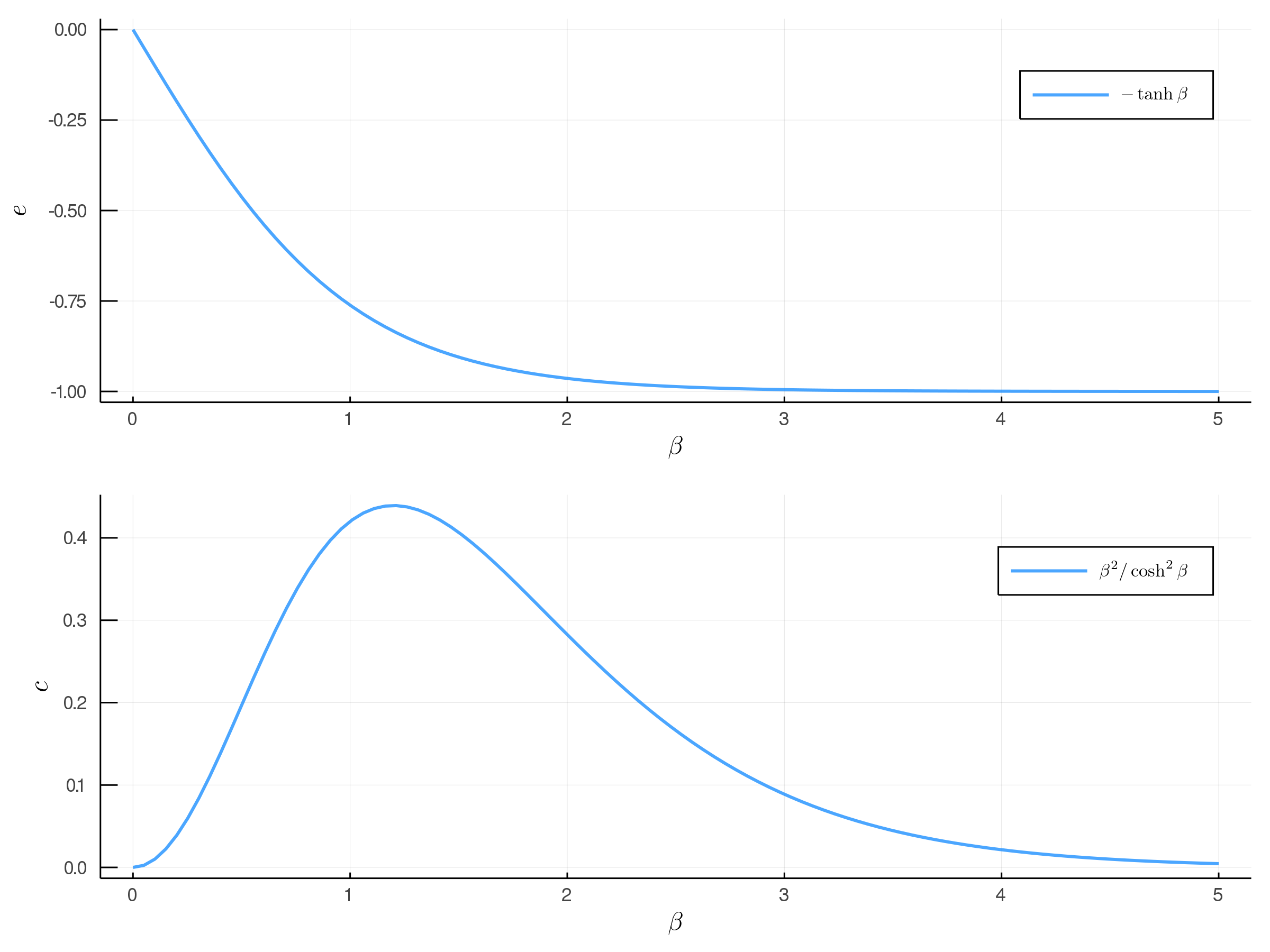
It is often useful to look at the energy and heat capacity on a per spin basis and in the thermodynamic limit ($N \rightarrow \infty$):
\[\begin{align*} \begin{split} e &= \frac{E}{N} \\ &= -J \bigg(1 - \frac{1}{N}\bigg) \tanh \beta J \\ \lim_{N \to \infty} e &= -J \tanh \beta J \end{split} \end{align*}\] \[\begin{align*} \begin{split} c &= \frac{C}{N} \\ &= k_B \beta^2 J^2 \bigg(1 - \frac{1}{N}\bigg) \frac{1}{\cosh^2 \beta J} \\ \lim_{N \to \infty} c &= k_B \beta^2 J^2 \frac{1}{\cosh^2 \beta J} \end{split} \end{align*}\]Below we plot the average energy and heat capacity per spin. We can see that for very low $\beta$ (high $T$) the energy is at its maximum of roughly zero, and decreases as $\beta$ increases ($T$ decreases). This makes sense with what we might think because at high temperatures we expect all of the spins to be anti-aligned and contribute the most to the energy whereas at low temperatures the spins all aligned contributing the least to the energy. The heat capacity can be seen to be roughly zero for very small $\beta$ due to the saturation effect (the system only has a finite number of energy states, thus at a certain point adding adding heat to the system will not increase the internal energy any more since there are no states with higher energy), and at higher $\beta$ we also observe a near zero heat capacity often seen in systems with an energy gap between the ground state and the first excited state.
Up Next
In multiple dimension ferromagnetic systems the Ising model becomes far too difficult to solve by analytical methods, thus this is where computational methods come in handy. Now that we have an idea of what the Ising model is we can begin our journey into simulating magnetism. In the next blog post we will discuss the basics of Markov Chain Monte Carlo (MCMC) methods which we will use to help us in our quest to understand more about Ferromagnetism.