Simulating Magnetism Part 3: Running an Ising Model Simulation
In this post we’ll cover how to implement an Ising model simulation using the previously discussed Metropolis algorithm. We will also see an annotated implementation of the Metropolis algorithm with some optimizations that help reduce the compute time. Once we have the simulation data we will plot it and analyze it for various temperatures and lattice sizes to see how the system behaves differently as those variables change.
MagSim.jl
In order to make the simulations easy to use and reproduce, it is convenient to put all of the code within a single package. This is why I created the Julia package MagSim.jl and open sourced it under the MIT license.
The main idea of the package is that there is magnetism models (e.g. Ising) and update algorithms (e.g. metropolis!).
For example, one can create an Ising model with $L = 32$ at the critical inverse temperature of $\beta_c = \log(1 + \sqrt{2}) / 2$ using the following:
julia> model = Ising(32, log(1 + √2) / 2)
Ising
L          = 32
β          = 0.3
n_sweeps   = 100000
start_type = cold
seed       = 8
q          = 0
The model by default is set to run $10^5$ update sweeps over the lattice (a sweep for a lattice with $N = L^2$ spins entails flipping $N$ spins).
To run the a simulation using the Metropolis algorithm we can use the metropolis! function.
This will perform the simulation and update the model, from which we can get the final numbers of the desired observables averaged over the simulation.
julia> metropolis!(model);
After the simulation is complete, we can access the statistics dictionary within the observables object of the model.
This dictionary contains a lot of information about the system (which can be accessed using the symbols listed after the quantity) such as the average energy per spin :e, average magnetization per spin :m, heat capacity per spin :c, magnetic susceptibility per spin :χ, as well as a couple others which will be discussed in later posts.
For example, to get the average energy value of the system:
julia> model.observables.statistics[:e]
-1.435243701171875
As a side note, these simulations use a seeded random number generator (seed value can be set with a kwarg to Ising), so these results are easy to replicate.
So far we’ve only covered a small portion of the package’s functionality, and we will cover more in future posts, but if you are interested in knowing more I encourage you to checkout the project on GitHub.
The code used to generate the data and plots in this post can be found here.
Metropolis Algorithm Implementation
Below is an annotated version of the metropolis! function from MagSim explaining the code, and some tips and optimizations.
As a side note, without loss of generality we can take $k_B = 1$ as well as $J = 1$ in our simulations which helps reduce the number of required numerical operations.
function metropolis!(model::Ising)
	# Due to the system thermalizing at first, we pick t₀ to be a number which before
	# we do not take observable measurements
	t₀   = floor(Int, model.params.cutoff * model.params.n_sweeps)
	# Since there are only several possible values ΔE can take on we pre-store these
	ΔE  = [-8, -4, 0, 4, 8]
	# To save time we precompute the exponential values we will use
	P = exp(-model.params.β) .^ ΔE

	# Loop n_sweeps over the lattice
	for t in 1:model.params.n_sweeps
		# Loop over each spin in the lattice sequentially along the columns
		for j in 1:model.params.L, i in 1:model.params.L
			# Convert ΔE to an index to use with ΔE and P
			k = Int(model.σ[i, j] * sum_of_neighbors(model, i, j) / 2 + 3)

			# Check whether or not to flip the spin, and flip it if so
			(ΔE[k] <= 0 || rand(model.rng) < P[k]) && (model.σ[i, j] *= -1)
		end

		# If the system is thermalized, then save the observables
		t > t₀ && update_observables!(model)
	end

	# Compute the final observables values, e.g. average energy
	compute_observables_statistics!(model)
end
Finite Size Effects
Now that we have an idea of how to run simulations using the package and extract information about the observables we can run some simulations to see how the system behaves. Before we do that though we need to get an idea of what finite size effects are.
When we are simulating a physical system, we often do so with finite size systems, e.g. in the simulation we ran above we used a lattice size of $L = 32 \implies N = 1024$. We often want to understand what the behavior is in the thermodynamic limit, i.e. $\lim\limits_{N \rightarrow \infty}$. This leads to a difference between what we actually simulate and what we’re actually looking for. One technique which can help us with this is running multiple simulations for different system sizes and see how the behavior of the system changes as the system size changes. From this we can extrapolate how the system behaves in the thermodynamic limit.
In the following sections we analyze the observables for various system sizes $L \in \{4, 8, 16, 32, 64\}$ and $\beta \in (0, 1]$.
Analyzing the Energy and Heat Capacity
Below we can see plots containing the average energy per spin $e$ and heat capacity per spin $c$ of the different system sizes at various inverse temperatures. For these simulations we estimate the heat capacity (to be specific, $C_V$ is the heat capacity at constant volume) using the following equation:
\[C_V = \frac{\partial \langle E \rangle}{\partial T} = k_B \beta^2 (\langle E^2 \rangle - \langle E \rangle^2)\]The above formula can be derived by using $\langle E \rangle = -\frac{\partial \log Z}{\partial \beta}$. Since our simulations are stochastic in nature we do not get an exact measure of the expectation value $\langle E \rangle$, rather we get the mean value $\overline{E}$ which is an estimator for the expectation value. Using that we compute the heat capacity with:
\[C = \beta^2 (\overline{E^2} - \overline{E}^2)\]And of course to put that on a per spin basis we take $c = C / L^2$.
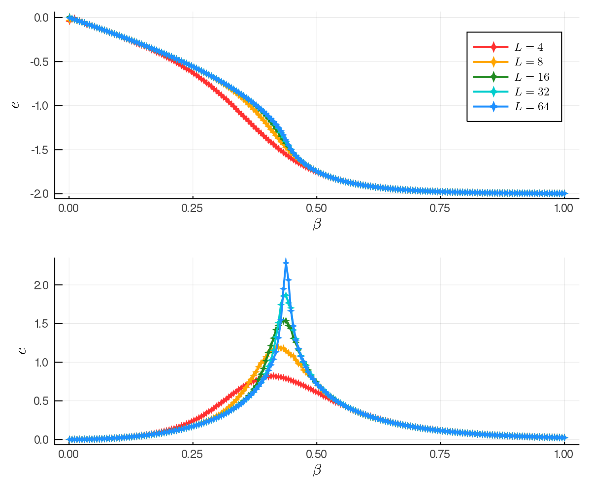
To add some context we recall this quote from the fist post in the series: “We can see that for very low β (high T) the energy is at its maximum of roughly zero, and decreases as β increases (T decreases). This makes sense with what we might think because at high temperatures we expect all of the spins to be anti-aligned and contribute the most to the energy whereas at low temperatures the spins all aligned contributing the least to the energy. The heat capacity can be seen to be roughly zero for very small β due to the saturation effect (the system only has a finite number of energy states, thus at a certain point adding adding heat to the system will not increase the internal energy any more since there are no states with higher energy), and at higher β we also observe a near zero heat capacity often seen in systems with an energy gap between the ground state and the first excited state.”
We also notice some other interesting behavior in the plots, namely the difference between the curves of the different lattice sizes. The difference in the system sizes is most apparent in the plot of the heat capacity. As the system size increases the peak of the heat capacity becomes much sharper and peaks at a much higher value. From this we can expect that in the infinite system size case the peak would almost look like a Dirac delta. The point around which it is peaking is the critical point (for 2D Ising systems this is $\beta = \log(1 + \sqrt{2}) / 2 \approx 0.44$), i.e. the point where the system transitions from the ordered low temperature phase to the disordered high temperature phase.
From visual inspection the energy curve also experiences something at the critical point, namely it’s an inflection point.
Analyzing the Magnetization and the Magnetic Susceptibility
The magnetization and magnetic susceptibility are plotted below. We recall from the first post in the series that the magnetization is the order parameter, which is a metric we can use to determine which phase the system is in. The magnetic susceptibility is a measure of how much the system would become magnetized when in an external magnetic field. The magnetic susceptibility is given by:
\[\chi = \frac{\partial \langle M \rangle}{\partial H} = \beta (\langle M^2 \rangle - \langle M \rangle^2)\]Which is estimated by:
\[\chi = \beta (\overline{M^2} - \overline{M})\]Note that we take the magnetic susceptibility per spin $\chi / L^2$.
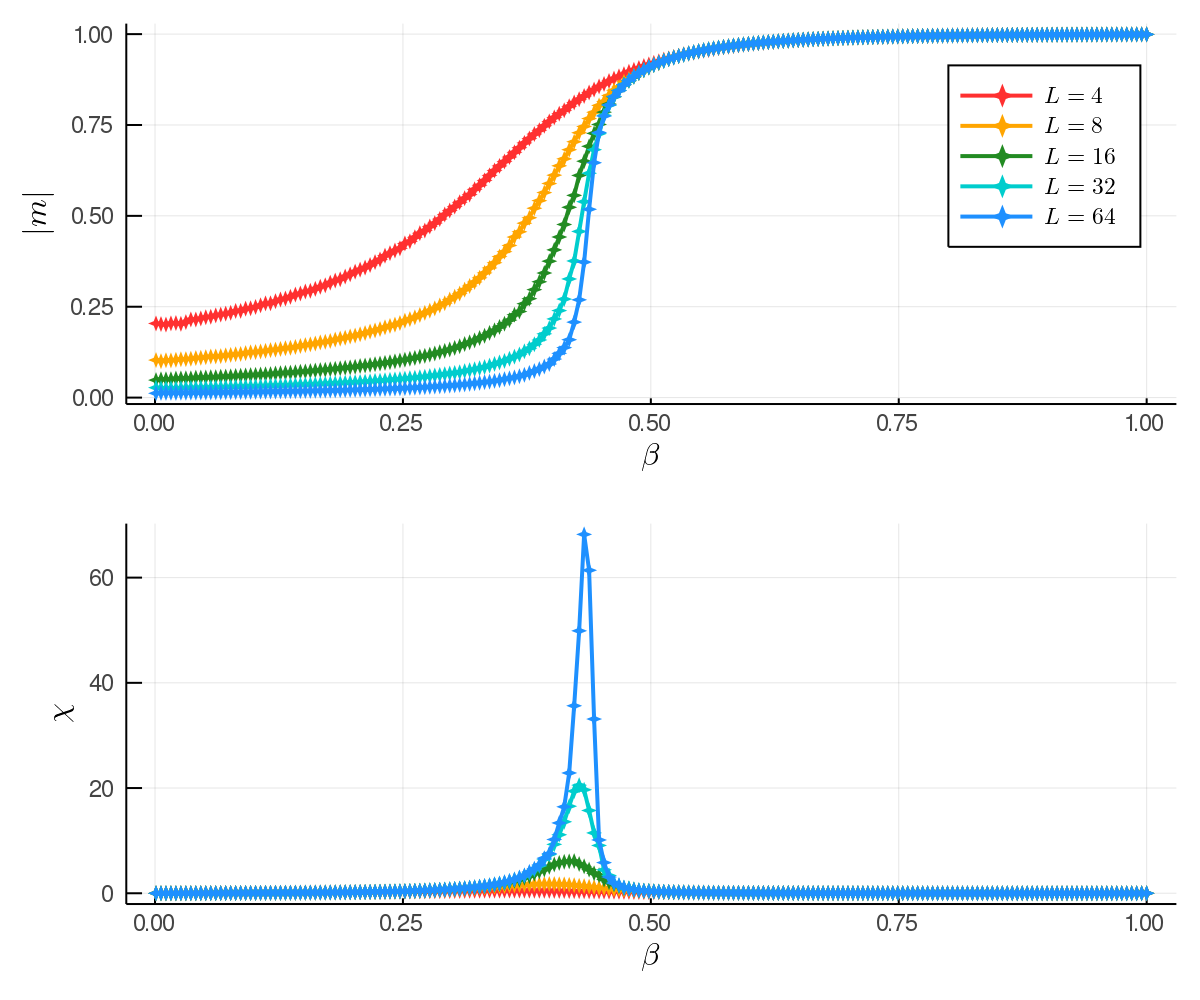
Looking at the plots we see that as the system size grows, the magnetization becomes more and more like what we would expect. At low beta we should see the order parameter near zero as the spins are in the disordered phase, and at high beta we expect to see the order parameter non-zero as the spins are in the ordered ferromagnetic phase.
This plot further illustrates the importance of taking finite size effects into account. It would be negligent to simulate just the smaller system and expect the macroscopic system to behave like that, thus to get the best idea of how the macroscopic system might act we should look at the largest system size and extrapolate the trend even further than that. From this we would expect the magnetization to look almost like a step function around the transition point.
The magnetic susceptibility exhibits a similar picture to that of the heat capacity; narrower and higher peaks as the system size increases, centered around the critical point.
Up Next
In this post we’ve seen how several key observables of a magnetic system behave at different temperatures and for different system sizes. I think one of the most important takeaways here is that we must always take into account the finite size effects when trying to understand the macroscopic system by studying finite size systems.
In the next blog post we will start on the q-state Potts model, which is a more generalized magnetism model than the Ising model, in which instead of spins only being able to take on one of two states they can take on one of q states instead.