An Interesting Problem
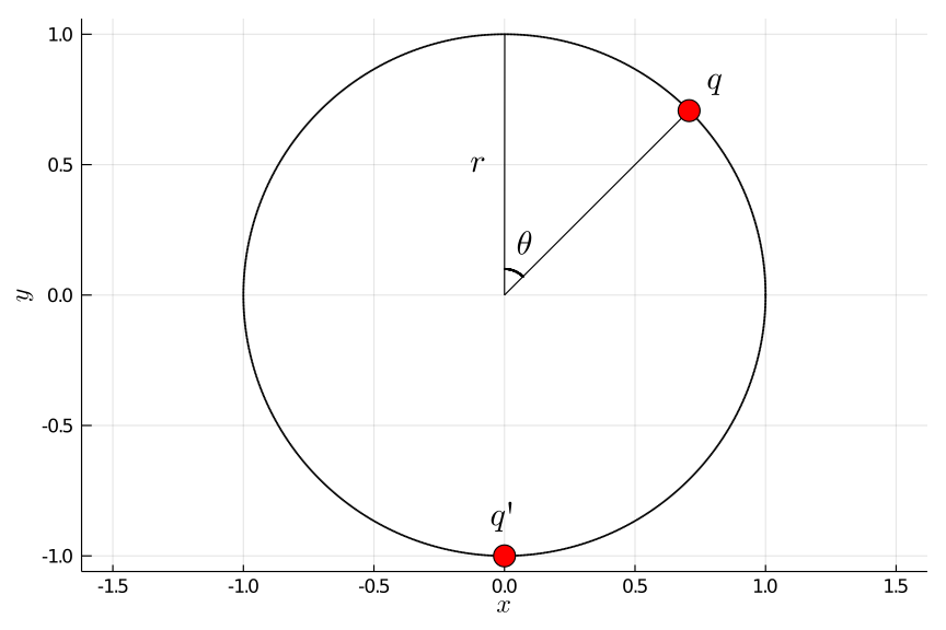
A few years ago one of my professors mentioned an interesting problem to me: take a charged particle located at $\mathbf{x}$ of charge $q$ confined to motion on a ring of radius $r$ with another charged particle at $\mathbf{x}’$ fixed at the bottom of the ring with a like charge $q’$. The charged particle that is allowed to move freely around the ring is subject to both the gravitational force as well as the Coulomb force generated by the electromagnetic interaction of the charges. In this post we’ll cover how to solve it and then animate it.
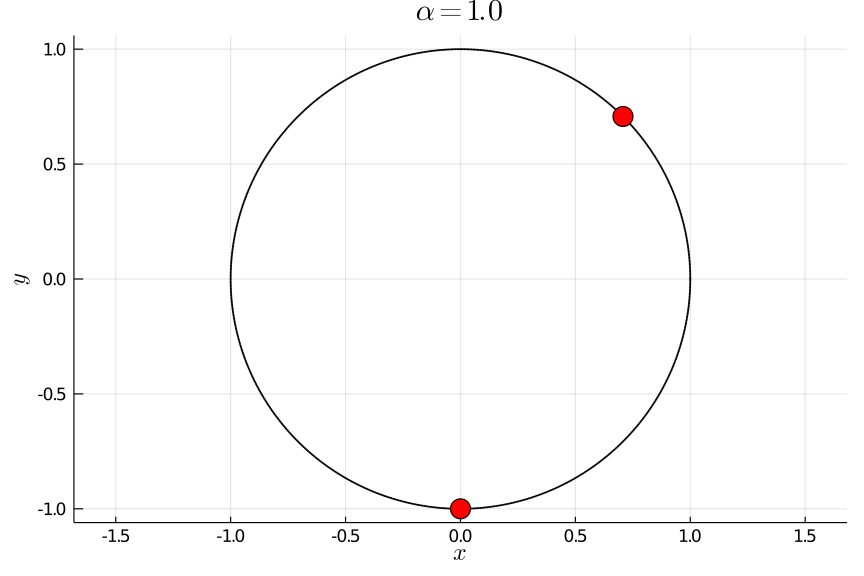
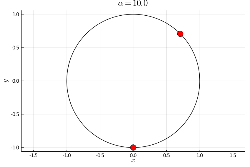
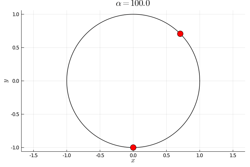
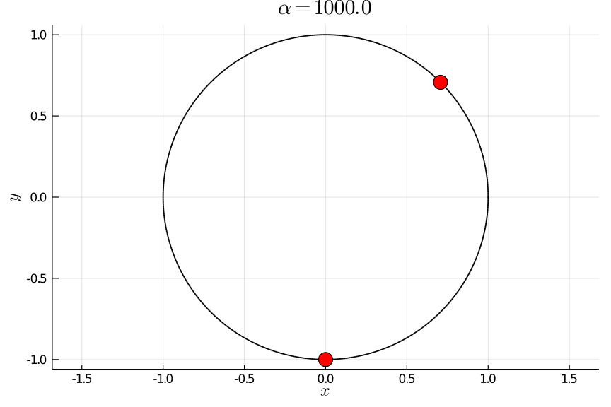
The system is illustrated in the image below.
A Solution Using Lagrangian Mechanics
We can solve this quite beautifully using Lagrangian mechanics. The Lagrangian $L$ is given by:
\[L = T - V\]where $T$ is the kinetic energy and $V$ is the potential energy. This problem can be modeled completely with one degree of freedom, that is the angle of displacement from the upright vertical position of the particle. We will use $\theta$ to denote this.
The kinetic energy is given by the rotational kinetic energy $\frac{1}{2} I \dot{\theta}^2$, and since it’s just a mass moving around the center at a distance $r$ the moment of inertia is given by $I = mr^2$, giving us:
\[T = \frac{1}{2} mr^2 \dot{\theta}^2\]The potential energy is the sum of the gravitational potential energy $V_g$ and the electric potential energy $V_e$:
\[\begin{equation} \begin{split} V_g &= mg\cos\theta \\ V_e &= \frac{1}{4\pi\epsilon_0}\frac{qq'}{||\mathbf{x} - \mathbf{x}'||} \end{split} \end{equation}\]We can compute the distance between the two particles using basic trigonometry:
\[||\mathbf{x} - \mathbf{x}'|| = 2r \sin\frac{\pi-\theta}{2} = 2r\cos\frac{\theta}{2}\]Giving us a potential energy of:
\[V = mg\cos\theta + \frac{\alpha}{\cos\frac{\theta}{2}}\]Where $\alpha = \frac{qq’}{8r\pi\epsilon_0}$. Thus our Lagrangian takes the form:
\[L = \frac{1}{2} mr^2 \dot{\theta}^2 - mg\cos\theta - \frac{\alpha}{\cos\frac{\theta}{2}}\]As discussed in a previous post, we can use the Lagrange-Euler equation to obtain a differential equation in $\theta$. We start by finding $\frac{\partial L}{\partial \theta}$:
\[\begin{equation} \begin{split} \frac{\partial L}{\partial \theta} &= mg\sin\theta - \frac{\alpha}{2} \frac{\sin\frac{\theta}{2}}{\cos^2\frac{\theta}{2}} \\ &= mg\sin\theta - \frac{\alpha}{2} \tan\frac{\theta}{2} \sec\frac{\theta}{2} \end{split} \end{equation}\]We then calculate $\frac{d}{dt}\Big[\frac{\partial L}{\partial \dot{\theta}}\Big]$:
\[\begin{equation} \begin{split} \frac{d}{dt} \bigg[\frac{\partial L}{\partial \dot{\theta}}\bigg] &= \frac{d}{dt} \bigg[ mr\dot{\theta} \bigg] \\ &= mr\ddot{\theta} \end{split} \end{equation}\]Combining the above into the Lagrange-Euler equation we obtain an expression for the angular acceleration:
\[\begin{equation} \begin{split} \frac{d}{dt} \bigg[\frac{\partial L}{\partial \dot{\theta}}\bigg] &= \frac{\partial L}{\partial \theta} \\ mr\ddot{\theta} &= mg\sin\theta - \frac{\alpha}{2} \tan\frac{\theta}{2} \sec\frac{\theta}{2} \\ \ddot{\theta} &= \frac{g}{r}\sin\theta - \frac{\alpha}{2mr^2} \tan\frac{\theta}{2} \sec\frac{\theta}{2} \end{split} \end{equation}\]Visualizing the System
Using numerical integration methods (here we will use velocity Verlet) we can simulate how the system will evolve over time. This allows us to obtain $\theta(t)$ which tells us everything we need to know. From this we can make an animation to visualize how the system behaves depending on how strong the charges are. We will use the quantity $\alpha$ (defined above) to control the charge interaction.
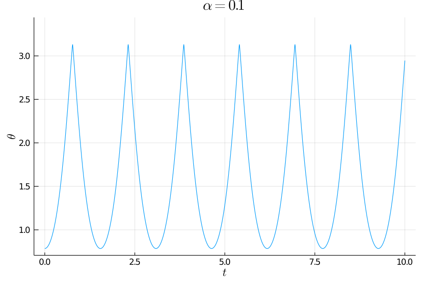
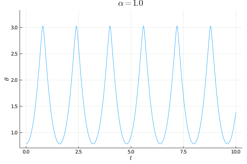
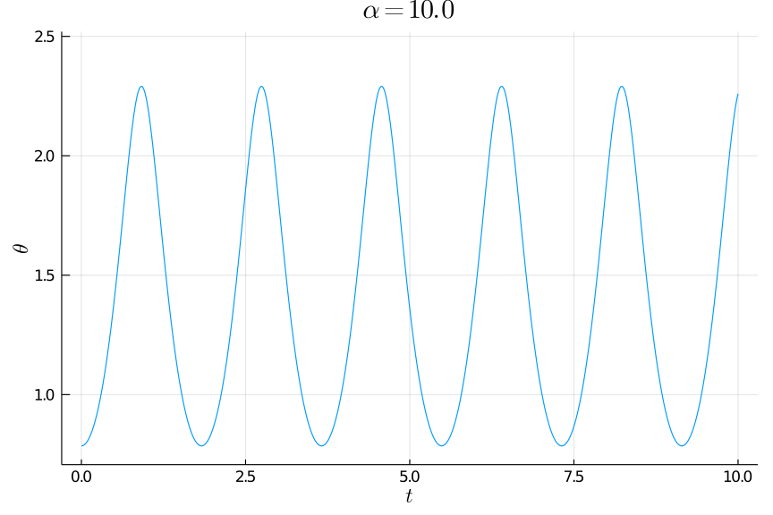
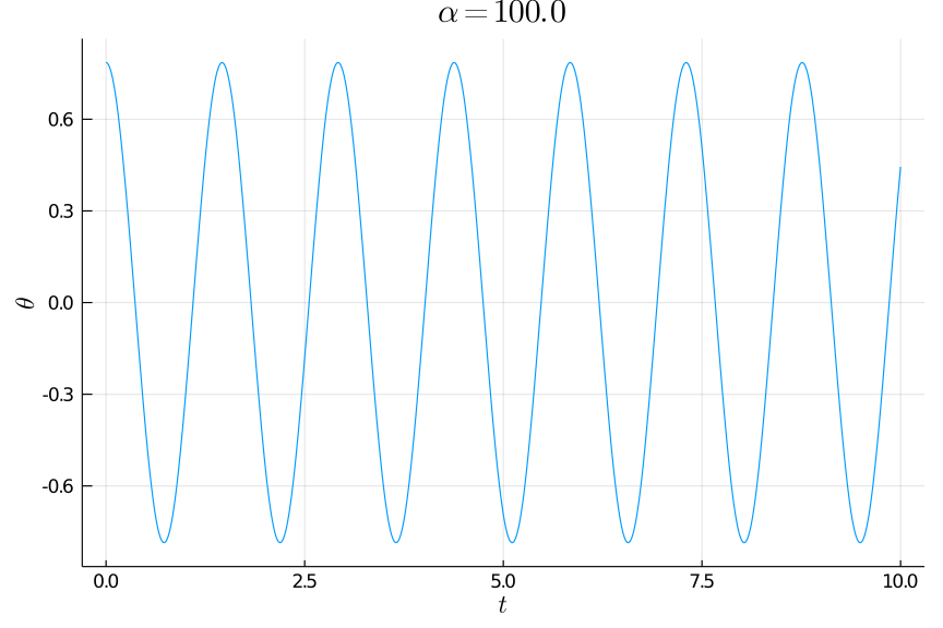
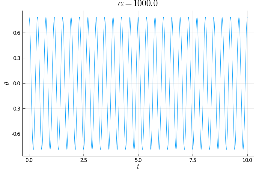
Below are animations for different values of $\alpha$, and below the animations are plots of $\theta$ as a function of time. All simulations were run with the initial conditions $\theta_0 = \frac{\pi}{4}, \dot{\theta}_0 = 0$. You can find the code here.
We can see in the first animation where $\alpha = 0.1$ that the particle oscillates about the right side of the ring and comes close to the particle at the bottom before being accelerated back up. The $\theta(t)$ plot shows sinusoidal-like behavior, but its upper peaks are much sharper than its lower ones, which tells us that it spends much less time near the fixed particle than near its other maximum $\theta_0$. The sharp upper peak is due to the inverse square dependence of the Coulomb force, because when two like-charged particles get close to each other the repulsive force between them becomes quite large. As we increase the value of $\alpha$ we observe that the free particle starts to stop further from the fixed particle, and the oscillations become more like a sine wave. After a certain point, the electric force overpowers that of gravity forcing the particle to oscillate about $\theta = 0$.
To describe this behavior in a more mathematical sense we can say for $\theta_0 \in (0, \pi), \dot{\theta}_0 = 0 \ \ \exists \ \alpha_0$ such that when $\alpha < \alpha_0$ the particle oscillates in the range $\theta \in [\theta_0, \theta_1]$ where $\theta_1 \in (\theta_0, \pi)$. When $\alpha \ge \alpha_0$ the particle oscillates in the range $\theta \in [-\theta_0, \theta_0]$. For $\alpha \ge \alpha_0$ the frequency of oscillation increases as $\alpha$ increases.