Simulating Magnetism Part 4: The $q$-State Potts Model
In this post we’ll go over what the $q$-State Potts model is, how the Metropolis algorithm can be applied to it, and see the results of running simulations with it.
The Potts Model
The Potts model is similar to the Ising model, but is more general in the sense that it allows the spins to take on $q$ different possible values rather than just two values as in the Ising model. We can think of these new possible spin states as vectors represented in polar coordinates with their orientation described by an angle $\theta_p = \frac{2\pi p}{q}$.
The energy in the Potts model (in the absence of an external magnetic field) is given by:
\[H = -J \sum_{\langle i j \rangle} \delta_{\sigma_i \sigma_j}\]Where $\delta_{ij}$ is the Dirac-$\delta$ which is equal to one if $i = j$ and zero otherwise. It’s important to note the difference from the Ising model in how the energy is quantized. In the Potts model a spin $\sigma_i$ has the possible local energy states of ${0, 1, 2, 3, 4}$, whereas in the Ising model the possible local energy states are ${-4, -2, 0, 2, 4}$
Now that we have a Hamiltonian, we’d also like an order parameter to keep track of the phase of the system. Let’s backtrack back to the Ising model where the magnetization per spin $m$ of the system is given by:
\[m = \frac{1}{N} \sum_i \sigma_i\]Now let $N_1$ be the number of spins with value $+1$ and $N_2$ be the number of spins with value $-1$, and we have that $N_1 + N_2 = N$ the total number of spins. We then let $n_p = N_p / N$, allowing us to represent the magnetization in a slightly different form:
\[m = \sum\limits_{p=1}^2 a_p^{(2)} n_p\]Where the coefficients $a_1^{(2)} = +1$ and $a_2^{(2)} = -1$ are the square roots of one. To generalize this to the Potts model we define our coefficients to be the $q$th roots of one, and our magnetization becomes:
\[m = \sum\limits_{p=1}^q a_p^{(q)} n_p = \sum\limits_{p=1}^q e^{\theta_p i} n_p\]Which yields a complex magnetization. The modulus and argument of this complex value represent the strength and orientation of the magnetization in the plane respectively.
Applying the Metropolis Algorithm
It’s quite straight forward to write a Metropolis algorithm for the Potts model. The only thing we really need to change from the one we wrote for the Ising model is how we compute the change in energy. Below is an implementation of the Metropolis algorithm which will run on the Potts model:
function metropolis!(model::Potts)
	# Due to the system thermalizing at first, we pick t₀ to be a number which before
	# we do not take observable measurements
	t₀ = floor(Int, model.params.cutoff * model.params.n_sweeps)
	# Since there are only several possible values ΔE can take on we pre-store these
	ΔE = -4:4
	# To save time we precompute the exponential values we will use
	P = exp(-model.params.β) .^ ΔE

	# Loop n_sweeps over the lattice
	for t in 1:model.params.n_sweeps
		# Loop over each spin in the lattice sequentially along the columns
		for j in 1:model.params.L, i in 1:model.params.L
			# Compute the spin value counts of the nearest neighbors
			# i.e. counts[q] = number of neighbors with spin value q
			counts   = compute_counts(model, (i, j))
			old_spin = model.σ[i, j]
			new_spin = rand(model.rng, UnitRange{Int8}(1, model.params.q))
			# Convert ΔE to an index to use with ΔE and P
			k        = (counts[old_spin] - counts[new_spin]) + 5

			# Check whether or not to flip the spin, and flip it if so
			(ΔE[k] <= 0 || rand(model.rng) < P[k]) && (model.σ[i, j] = new_spin)
		end

		# If the system is thermalized, then save the observables
		t > t₀ && update_observables!(model)
	end

	# Compute the final observables values, e.g. average energy
	compute_observables_statistics!(model)
end
Analyzing the Energy and Heat Capacity
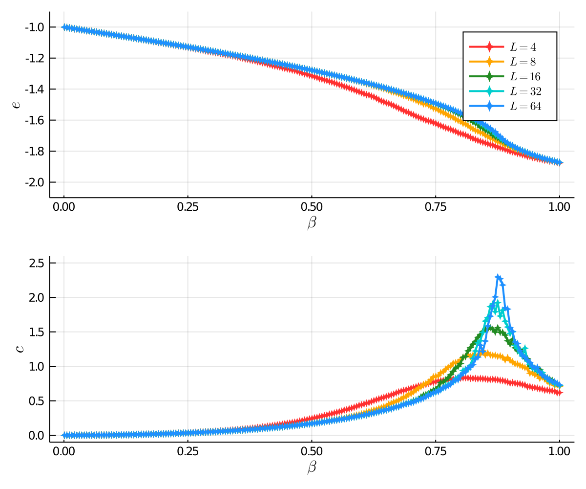
We take a look at the case where $q = 2$ so that we can compare our results to the Ising model. In the plot below we have the energy and heat capacity, where we can see that the overall curves exhibit similar behavior to the Ising model except shifted to the right where the critical point is now $\beta_{c, \text{Potts}} = 2 \beta_{c, \text{Ising}} = \ln(1 + \sqrt{2}) \approx 0.88$.
We’ll keep this post short due to the fact that we have a more interesting model to study in the next post.
Up Next
In the next blog post we’ll introduce the XY model, where the spins are allowed to take any orientation in a plane, and see how it undergoes a unique phase transition.